This page contains a quick tutorial for the main pandda programs, as well as a more detailed walkthrough.
Quick Tutorial
For those in a hurry, below is a minimal demonstration of the PanDDA implementation using an example dataset.
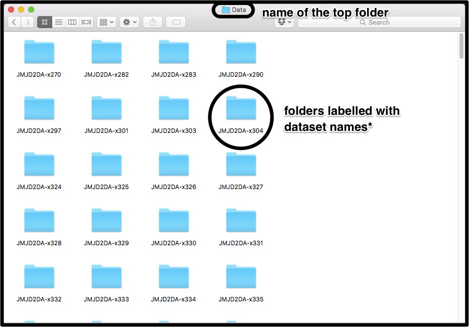
Download the example dataset of bromodomain adjacent to zinc finger 2b (baz2b) from zenodo: data.zip. This contains 201 datasets soaked with different compounds from fragment screening experiments. Download the zipfile into a folder and unzip it. Inside the unzipped folder, the data are organised into folders labelled with the dataset name. Inside each sub-folder are the raw crystallographic data and the data after refinement with dimple (from CCP4).
The PanDDA workflow of pandda.analyse ⇢ pandda.inspect ⇢ pandda.export is described below.
In the terminal, go to the directory containing the unzipped folder called data.
To run a full PanDDA analysis of all datasets, run the command
pandda.analyse data_dirs='./data/*' pdb_style='*.dimple.pdb' cpus=X
where you should replace
To run a shorter analysis - taking about an hour using seven cpus - run the command
pandda.analyse data_dirs='./data/*' pdb_style='*.dimple.pdb' cpus=X \
    high_res_upper_limit=1.8 high_res_lower_limit=1.8 dynamic_res_limits=False
This will only analyse datasets with a resolution higher than 1.8Å, and will analyse all datasets at 1.8Å.
After the (short) analysis has finished, the logfile should end with something like
############################################## <~~~> ###############################################
###                                      ANALYSIS COMPLETE                                       ###
############################################## <~~~> ###############################################

Total Analysis Time: 00 hours:26 minutes:56 seconds

############################################## <~~~> ###############################################
###                            Writing PanDDA End-of-Analysis Summary                            ###
############################################## <~~~> ###############################################

----------------------------------->>>
Collating Clusters
------------------------------------->>>
Dataset BAZ2BA-x434: 1 Events
Dataset BAZ2BA-x448: 1 Events
Dataset BAZ2BA-x451: 1 Events
Dataset BAZ2BA-x463: 2 Events
Dataset BAZ2BA-x480: 1 Events
Dataset BAZ2BA-x481: 1 Events
Dataset BAZ2BA-x489: 1 Events
Dataset BAZ2BA-x492: 1 Events
Dataset BAZ2BA-x503: 1 Events
Dataset BAZ2BA-x529: 1 Events
Dataset BAZ2BA-x538: 1 Events
Dataset BAZ2BA-x556: 1 Events
Dataset BAZ2BA-x559: 1 Events
Dataset BAZ2BA-x603: 1 Events
Dataset BAZ2BA-x612: 1 Events
Dataset BAZ2BA-x614: 1 Events
------------------------------------->>>
Total Datasets with Events: 16
Total Events: 17
------------------------------------->>>

------------------------------------->>>
Potentially Useful Shortcuts for Future Runs
------------------------------------->>>
All datasets with events:
exclude_from_characterisation=BAZ2BA-x434,BAZ2BA-x448,BAZ2BA-x451,BAZ2BA-x463,BAZ2BA-x480,BAZ2BA-x481,BAZ2BA-x489,BAZ2BA-x492,BAZ2BA-x503,BAZ2BA-x529,BAZ2BA-x538,BAZ2BA-x556,BAZ2BA-x559,BAZ2BA-x603,BAZ2BA-x612,BAZ2BA-x614
------------------------------------->>>
Datasets with events at Site 1
exclude_from_characterisation=BAZ2BA-x434,BAZ2BA-x451,BAZ2BA-x480,BAZ2BA-x481,BAZ2BA-x492,BAZ2BA-x529,BAZ2BA-x538,BAZ2BA-x559
------------------------------------->>>
Datasets with events at Site 2
exclude_from_characterisation=BAZ2BA-x448,BAZ2BA-x489,BAZ2BA-x556,BAZ2BA-x603
------------------------------------->>>
Datasets with events at Site 3
exclude_from_characterisation=BAZ2BA-x503,BAZ2BA-x614
------------------------------------->>>
Datasets with events at Site 4
exclude_from_characterisation=BAZ2BA-x463
------------------------------------->>>
Datasets with events at Site 5
exclude_from_characterisation=BAZ2BA-x612
------------------------------------->>>
Datasets with events at Site 6
exclude_from_characterisation=BAZ2BA-x463
------------------------------------->>>

------------------------------------->>>
Lists of datasets used to generate the statistical maps
------------------------------------->>>
Statistical Electron Density Characterisation at 1.8A
> Density characterised using 60 datasets
> Dataset IDs:
    BAZ2BA-x425,BAZ2BA-x427,BAZ2BA-x428,BAZ2BA-x430,BAZ2BA-x431,
    BAZ2BA-x433,BAZ2BA-x434,BAZ2BA-x440,BAZ2BA-x442,BAZ2BA-x446,
    BAZ2BA-x448,BAZ2BA-x449,BAZ2BA-x451,BAZ2BA-x452,BAZ2BA-x453,
    BAZ2BA-x454,BAZ2BA-x455,BAZ2BA-x458,BAZ2BA-x459,BAZ2BA-x463,
    BAZ2BA-x472,BAZ2BA-x475,BAZ2BA-x477,BAZ2BA-x479,BAZ2BA-x480,
    BAZ2BA-x481,BAZ2BA-x485,BAZ2BA-x486,BAZ2BA-x487,BAZ2BA-x488,
    BAZ2BA-x489,BAZ2BA-x492,BAZ2BA-x494,BAZ2BA-x495,BAZ2BA-x496,
    BAZ2BA-x497,BAZ2BA-x500,BAZ2BA-x501,BAZ2BA-x503,BAZ2BA-x505,
    BAZ2BA-x506,BAZ2BA-x508,BAZ2BA-x510,BAZ2BA-x511,BAZ2BA-x512,
    BAZ2BA-x515,BAZ2BA-x516,BAZ2BA-x518,BAZ2BA-x519,BAZ2BA-x520,
    BAZ2BA-x521,BAZ2BA-x525,BAZ2BA-x526,BAZ2BA-x527,BAZ2BA-x528,
    BAZ2BA-x529,BAZ2BA-x530,BAZ2BA-x532,BAZ2BA-x535,BAZ2BA-x537
------------------------------------->>>
Writing final output files

----------------------------------------------- *** ------------------------------------------------
---                                     Writing output CSVs                                      ---
----------------------------------------------- *** ------------------------------------------------

------------------------------------->>>
Writing Dataset + Dataset Map Summary CSVs
    /path/to/folder/pandda/analyses/all_datasets_info.csv
    /path/to/folder/pandda/analyses/all_datasets_info_maps.csv
    /path/to/folder/pandda/analyses/all_datasets_info_masks.csv
------------------------------------->>>
Writing COMBINED Dataset Summary CSV
    /path/to/folder/pandda/analyses/all_datasets_info_combined.csv
------------------------------------->>>
Writing Event+Site Summary CSVs
    /path/to/folder/pandda/analyses/pandda_analyse_events.csv
    /path/to/folder/pandda/analyses/pandda_analyse_sites.csv
------------------------------------->>>
Datasets analysed at each resolution:
====================================================================>  127  1.8
------------------------------------->>>


------------------------------------->>>
Datasets Analysed: 127
Datasets that could have been analysed: 200
------------------------------------->>>

Runtime: 00 hours:35 minutes:16 seconds

############################################## <~~~> ###############################################
###                            .. FINISHED! PANDDA EXITED NORMALLY ..                            ###
############################################## <~~~> ###############################################

------------------------------------->>>
Writing dataset information for any future runs
Adding information about 0 new datasets (on future runs these will be known as "old" datasets).
Pickling Object: pickled_data/dataset_meta.pickle
If you get this then we can now proceed to model the identified ligands.
Change into the newly created pandda output directory and open pandda.inspect:
cd pandda
pandda.inspect
This will open up a coot modelling window and a PanDDA window.
Since the ligand files were present in the input data directories, these are automatically detected by PanDDAs and the ligand is loaded and placed into the middle of the screen.
Model the ligand as normal and delete/re-model any waters that do not match the loaded electron density maps. Don't forget to click the Merge Ligand button to merge the modelled ligand with the protein model.
You can use the buttons and text boxes at the bottom of the PanDDA window to record information about whether a ligand was fitted, and to record any comments about the ligand modelling.
Click >>> Next >>> (Save Model) to save the model and move to the next event. Model as many ligands as you wish.
Show Summary opens a summary of the PanDDA analysis. Click Quit to update the output and exit.
After modelling is finished, the structures can be exported for refinement. Change into the directory containing the pandda folder and run the command
pandda.export pandda_dir='./pandda'
This will generate a new folder called pandda-export, containing the datasets where a model was built. The output structures for each dataset are a combination of bound-state models generated in the previous step, and the input structures from dimple (the unbound state). These multi-state ensembles naturally allows the bound and unbound states of the protein to be represented in the model; ligands will rarely - if ever - bind at unitary occupancy, so the unbound state of the crystal should be present in the model.
Models can be quickly and easily refined using the script giant.quick_refine.
giant.quick_refine program=refmac model.pdb model.mtz ligand.cif
You can create parameter files that allow the occupancy of the superposed states to be constrained during refinement using (these are created automatically by pandda.export by default)
giant.make_restraints model.pdb
Occupancy parameter files can be passed to giant.quick_refine by using
giant.quick_refine program=refmac model.pdb model.mtz ligand.cif parameters.params
For the first round of refinement after pandda.export, make sure you use the XXX-ensemble-model.pdb and XXX-pandda.input.mtz for refinement.
More information about modelling and refinement can be found in the walkthrough below.
Standard PanDDA protocol walkthrough
For those not in a hurry, below is a longer walkthrough that describes all major steps of a PanDDA analysis.
The pandda suite is composed of three main programs:
- pandda.analyse:
- Largest component of the program. Does most of the processing of the data.
- pandda.inspect:
- Allows the user to inspect and manually model the processed datasets with coot.
- pandda.export:
- Processes the modelled structures and generates bound-unbound ensembles for refinement.
The main workflow of the program (pandda.analyse ⇢ pandda.inspect ⇢ pandda.export) will be described in more detail below.
The terminology that is used throughout this page is described below.
| Dataset | A PDB and corresponding MTZ file. |
|---|---|
| Reference Dataset | The dataset to which all other datasets (both structures and maps) are aligned for analysis. Normally the highest resolution dataset. |
| Ground State Crystal | The "normal" state of the crystal. May be referred to as the "apo" crystal or the "unbound" crystal, but this is not necessarily the case, as the ground state could include bound buffer molecules, or a substrate, etc. PanDDA detects differences between individual datasets and the "ground state crystal" defined by the ensemble of datasets. |
| Events | "Events" are differences between crystals and the ground state crystal. These may be binding ligands, binding metals, stochastic movements in the crystal, shifts in crystal contacts, or anything else. |
The next couple of sections refer to datasets from another fragment screen that can be found on zenodo (here), or you can download the required data directly: data.zip.
However, these sections only discuss the different ways of selecting datasets, so it is not necessary to download and analyse this dataset. The modelling examples in the later sections return to the BAZ2B dataset used in the first tutorial. Sorry for any confusion.
The input to panda.analyse is a series of refined datasets, sorted into folders — one for each dataset.
Each folder needs to contain a minimum of 2 files (and possibly the ligand files):
- Refined PDB file
- Refined MTZ file
- Ligand PDB file (optional)
- Ligand CIF file (optional)
All Refined PDB files must contain roughly the same protein model (same number and ordering of protein chains), but the composition of the models may vary: residues may be missing in some datasets (e.g. at the terminus of a chain); alternate conformations of residues may differ; and models may have different solvent models. However, for best results the models should be as similar as possible. Input models are best obtained using a refinement pipeline such as Dimple, where all datasets consist of the same reference structure refined against new sets of diffraction data.
The first thing that pandda.analyse needs to be told is which folders (datasets) to process, and how they should be labelled. This is passed to pandda.analyse as:
pandda.analyse data_dirs='./path/to/directory/*'
pandda.analyse uses the parts of the filepath captured by the * to label the datasets.
In the example above, where ./path/to/directory contains folders called JMJD2DA-x001, JMJD2DA-x002, JMJD2DA-x003, etc, datasets will be labelled
JMJD2DA-x001, JMJD2DA-x002, JMJD2DA-x003, ...
However, if we had run:
pandda.analyse data_dirs='./path/to/directory/JMJD2DA-*'
the datasets would have been labelled
x001, x002, x003, ...
The default output folder from pandda.analyse is "./pandda". However, this can be changed by using:
pandda.analyse ... out_dir='./output_folder'
The next step is to pick up the files within each of the folders. The files in the folders can be named however you want, as long as they’re named consistently.
In this example, the files come from dimple, and all of the files in all of the datasets are labelled the same (final.pdb, final.mtz):
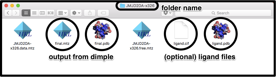
To pick these files up, we use the command line flags:
pandda.analyse ... pdb_style='final.pdb' mtz_style='final.mtz' lig_style='ligand.cif'
If the mtz files are labelled the same as the pdb files, except for the change from ".pdb" to ".mtz", then the mtz_style flag can be left out. The "ligand.pdb" file will be picked up automatically, as long as it is named the same as the "ligand.cif" file, except for the change from ".cif" to ".pdb".
To pick up all "cif" files in a directory, simply use lig_style="*.cif". Therefore, we could also use:
pandda.analyse ... pdb_style='final.pdb' lig_style='*.cif'
These filenames are the defaults of the program, so actually these options can be omitted in this case...
In this example, the files again come from dimple, but now all of the files are named using the dataset label:
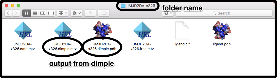
To pick these files up, we use the command line flags:
pandda.analyse ... pdb_style='*.dimple.pdb' mtz_style='*.dimple.mtz'
Again, if the mtz files are labelled the same as the pdb files, the mtz_style flag can be left out. The ligand files are covered in the previous example.
The part of the filename captured by the * must be the same as the part captured by the * in the folder name. E.g. for a file XXX.dimple.pdb in folder XXX, pdb_style="*.dimple.pdb" rather than "*.pdb" or anything else.
So, the final command would be:
pandda.analyse ... pdb_style='*.dimple.pdb'
Now we will cover the classification of datasets, which affects how they are processed by pandda.analyse. There are several flags that control how datasets are treated:
exclude_from_characterisation
Exclude datasets from calculation of the mean map, and other statistical maps. This flag is most commonly used when the dataset is known to contain a bound ligand, or to be a noisy dataset.
exclude_from_z_map_analysis
Exclude datasets from analysis. This is normally used when the dataset is known not to contain a bound ligand, and simply saves time in the running of the program.
ground_state_datasets (v0.3 only)
Define a set of \emph{known} ground-state datasets to be used for characterisation. All other datasets will be excluded from characterisation. This is used when you have a set of known ground-state datasets and a set of putative bound datasets that you are screening.
ignore_datasets
Exclude datasets completely. pandda.analyse will not process this folder at all.
The options that are given to these flags are a comma-separated list of dataset labels (e.g. option="label1,label2,label3,...").
Example:
For datasets that are labelled by folder names as above (JMJD2DA-x001, JMJD2DA-x002, ...), say we want to exclude datasets JMJD2DA-x005 and JMJD2DA-x015 from building, and dataset JMJD2DA-x099 from analysis. This is done by:pandda.analyse ... exclude_from_characterisation="JMJD2DA-x005,JMJD2DA-x015" exclude_from_z_map_analysis="JMJD2DA-x099"
(Note that there are no spaces around the commas)
All datasets that are not selected with the exclude_from_characterisation or exclude_from_z_map_analysis flags will be used for both building and analysis.
For help on running an analysis where you don't know which datasets are ground-state datasets, take a look at the strategies page.Here are some other useful parameters that control the running of the program:
- cpus=<num>
- Select the number of cpus to run the program on.
- dataset_prefix=<label>
- Add a prefix to the labelled datasets. dataset_prefix="prefix-" would cause "x001" to become "prefix-x001".
Once the analysis has been run, we model the identified events using pandda.inspect.
We now return to the BAZ2B dataset from the first tutorial...
After pandda.analyse has been run, we need to inspect and model the bound ligands that have been identified.
The modelling is done in pandda.inspect.
First, you need to be in the pandda.analyse output directory (normally named "pandda")
cd ./path/to/directory/pandda
and then simply type
pandda.inspect
This will open coot with a custom pandda-inspect window that controls the navigation through the potential hits identified by pandda.analyse. Relevant structures and electron density maps are loaded automatically as required. You can also record comments and meta-data about each identified event, and about each site (a group of events).
Navigating through the results: Interesting events are grouped into sites by their position on the protein surface, and pandda.inspect allows you to navigate these events sequentially, or to jump to a particular site. You can also jump to datasets that haven't been viewed before, or only jump to datasets where something has been modelled.
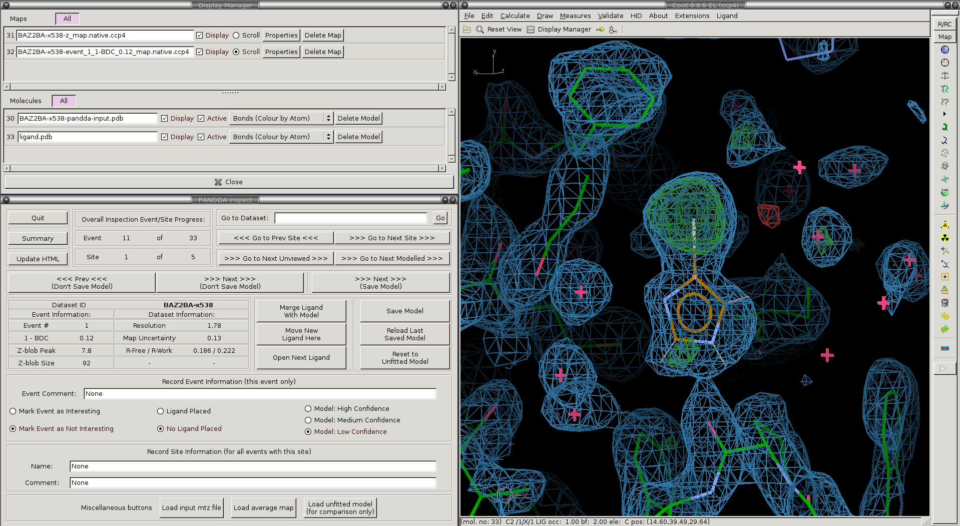
The pandda.inspect windows: The window in the lower-left allows navigation between events in different datasets, displays information about the loaded dataset and event, and allows you to record comments about each event. The normal coot file-window in the upper-left shows which files are open, and allows you to toggle the different maps on and off as required. The normal coot modelling-window, right, allows the modelling of the ligand. As you navigate through the events, relevant files are opened and loaded automatically.
The files loaded for each dataset and the buttons in the pandda GUI are described below:
We will now go through and describe each of the files that pandda.inspect loads up for each dataset:
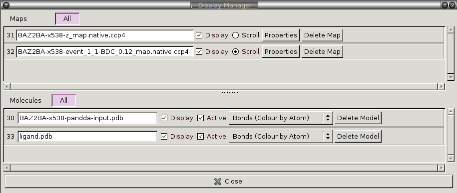
Loaded Electron Density Maps:
| <label>-z_map.native.ccp4 | Shows the extent of deviations from the ensemble of crystallographic datasets. Large positive or negative Z-scores (±3) indicate significant deviations from the ensemble, and may represent interesting features. |
|---|---|
| <label>-event_X_1-BDC_Y_map.native.ccp4 | Partial-difference density obtained by subtracting a fraction of the mean map from the dataset map. This reveals the density for low-occupancy binding events. X indicates which event in this dataset is being inspected, and Y indicates the amount of mean map that has been subtracted (amount subtracted = 1-Y). |
Loaded Structures:
| <label>-pandda-input.pdb | The input structure to pandda.analyse for this dataset. This is loaded until a *-pandda-model.pdb is created, which is then loaded instead. |
|---|---|
| <label>-pandda-model.pdb | Any changes made to <label>-pandda-input.pdb will be saved to this file. This is the structure that will then be loaded for any future inspection of the dataset. |
| ligand files | These will be automatically loaded if they were provided to pandda.analyse. The ligand will be placed in the centre of the screen. If <label>-aligned-structure.pdb is loaded, then the ligand will be displayed, but if <label>-pandda-model.pdb is loaded, then the ligand is hidden. |
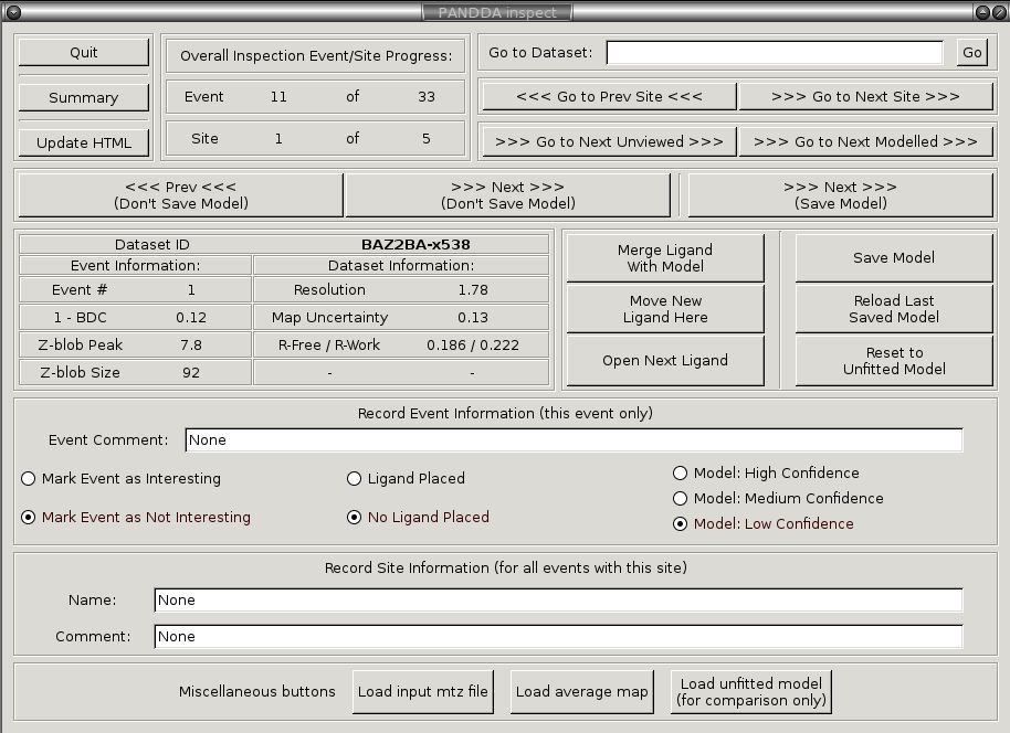
General |
|
|---|---|
Quit |
Safely quit pandda.inspect, saving all meta-data from the gui. |
Summary |
Load summary of the inspection in a new window, allowing to see the overall status. pandda.inspect will be frozen until this window is closed. |
Navigation |
|
>>> Next >>> (Save Model) |
Navigate to the next identified event, saving the current model (all meta-data is also saved). |
>>> Next >>> (Don't Save Model) |
Navigate to the next identified event, not saving the current model (all meta-data is still saved). |
<<< Prev <<< (Don't Save Model) |
Navigate to the previous identified event, not saving the current model (all meta-data is still saved). |
>>> Go to Next Site >>> |
Navigate to the first event of the next site, not saving the current model (all meta-data is still saved). |
<<< Go to Prev Site <<< |
Navigate to the first event of the previous site, not saving the current model (all meta-data is still saved). |
>>> Go to Next Unviewed >>> |
Navigate to the next not-previously-inspected event (all meta-data is still saved). |
>>> Go to Next Modelled >>> |
Navigate to the next modelled event - events where a model of the protein has been saved - (all meta-data is still saved). |
Modelling |
|
Move Ligand Here |
Move the ligand to the centre of the screen (even if it is not displayed) - this only works with the automatically loaded ligand file. |
Merge Ligand with Model |
Merge the open ligand file with the protein model (either the <label>-aligned-structure.pdb or <label>-pandda-model.pdb) - this only works with the automatically loaded ligand file |
Save Model |
Save the currently open structure of the protein (either the <label>-aligned-structure.pdb or <label>-pandda-model.pdb). |
Reset model |
Reload the last saved model of the protein (either the <label>-aligned-structure.pdb or <label>-pandda-model.pdb, depending on whether any modelling had previously been done). Any changes made since the last save will be lost. |
Recording Data |
|
Mark Interesting/Mark Not Interesting |
Mark the event as a crystallographically interesting event (not noise). It might be a binding ligand, or a random loop reordering. Either way, mark it if it is something worth noting. Marking something as interesting will not cause anything to happen, so it is ok to be liberal in marking events as interesting. |
High/Medium/Low Confidence |
Record the confidence in the built model. If it is a ligand being modelled: Is the ligand definitely there? Or only probably? Or is there definitely a ligand there but the identity is uncertain? Or is it just a tentative model? |
Ligand Placed/No Ligand Placed |
Has a ligand been added to the model? Recording of whether a ligand has been placed is not automatic. |
In the pandda paradigm, we are not trying to model the full crystallographic dataset, but only the new, minor, conformation of the protein.
Focus on areas that exhibit large Z-scores in the
Only model the conformation of the protein that is present in the event map.
There are several things that need to be done to achieve the best results from using panddas:
| 1) | Prune solvent molecules and alternate sidechain conformations | Delete those atoms and alternate conformations that are not present in the event map. |
|---|---|---|
| 2) | Fix conformations and rotamers that have changed | For those residues where the sidechain conformation or water molecule position has changed, simply correct the model as would be normal practice. Add new alternate conformers where necessary. |
| 3) | Model the ligand (if present) and add new solvent molecules. | Add new solvent molecules to the protein model where required. The ligand should already be loaded if it was supplied to pandda.analyse. You can move it to the centre of the screen using the Move new ligand here button, and you can merge it with the model using the Merge new ligand button. |
| 4) | Save the changes to the model. | If you want to save the changes to the model you can use the Save Model button. Or, if you use the >>> Next Event >>> (Save Model) button, the model will be saved and the next dataset will be loaded. |
These steps are demonstrated in the example below:
What follows is a demonstration of ligand modelling for a ligand in the BAZ2B dataset (from the tutorial at the top of the page).
We begin where the event has just been loaded in pandda.inspect. The loaded structures and maps are loaded as described in the previous section.
The ligand is displayed and moved to the centre of the screen - no attempt is made to fit the ligand into the density.
It is important to note that the maps are pre-scaled to absolute or sigma-like values. This means that the "rmsd" value reported by coot is meaningless. The number printed next to the rmsd value (in e/Å^3) is actually the correct contour level of the map.
For sigma-scaled maps (the default), the sigma-level of the Event map is determined by taking this number and dividing by (1-BDC). So a 1-BDC value of 0.1, and a map level of 0.2 leads to a sigma level of 2.
> The Z-Map is displayed at a contour of ±3
> The Event map is displayed at a contour of 2σ.
To aid the convergence of occupancy refinement, the occupancy of the ligand is set to 2*(1-BDC) (this is an empirical estimation of the occupancy) and the B-factors of the ligand are set to 20.
A newly-opened event in pandda.inspect:
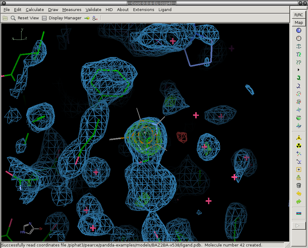
1) Prune solvent molecules and superfluous sidechain conformations.
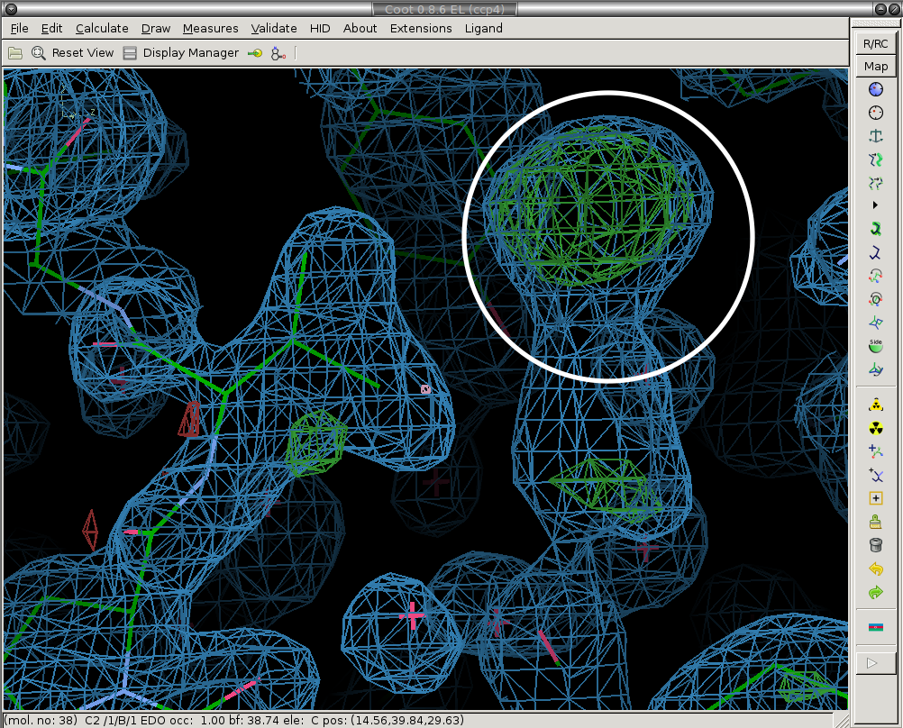
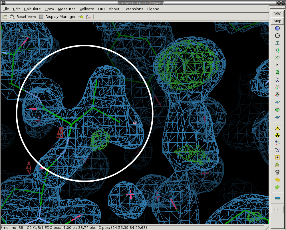
The first step is to delete the solvent molecules that have disappeared from the ground-state model (are not present in the bound state).
We delete the ethylene glycol circled in white.
Before:
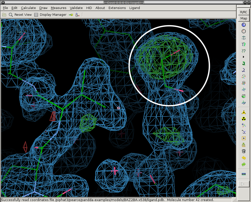
After:
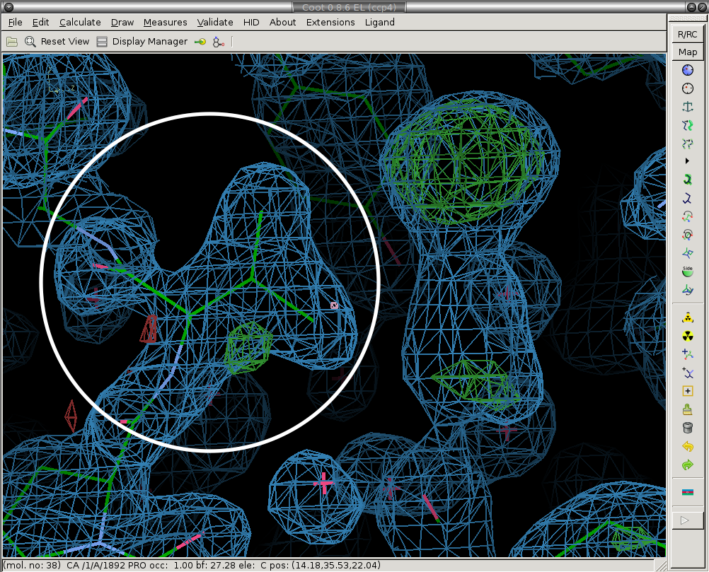
2) Fix conformations and rotamers that have changed.
Next we re-model the parts of the structure that have moved. We real-space refine the conformers that have moved (circled in white).
Before:
After:
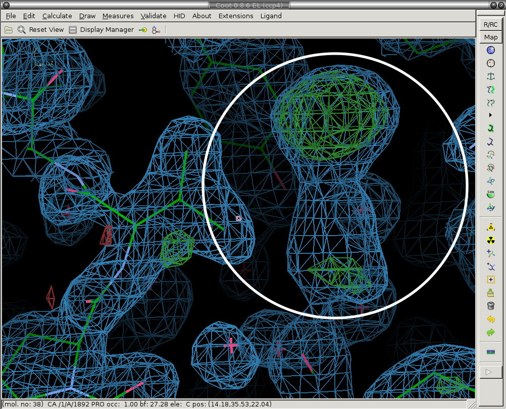
3) Model the ligand (if present) and new solvent molecules.
We place the ligand and merge it with the protein molecule ("Merge Ligand" button). Ligand is circled in white. Here you should also add new water (or other solvent molecules as necessary).
Before:
After:
4) Save the changes to the model.
Finally, we move to the next model (using the "Next, Save Model" button), and the current model is saved automatically.
Once all of the models have been built, we prepare the models for crystallographic refinement using pandda.export.
There are three results pages that are generated by pandda.analyse and pandda.inspect. They can be accessed from within pandda.inspect by clicking on the summary button, or by typing pandda.show_summary whilst in the pandda output directory.
1) pandda.analyse input summary.
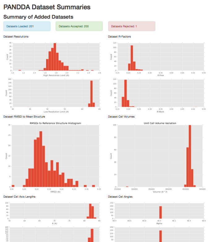
Graphs representing the distributions of varied parameters across the datasets.
- Unit cell size and angles distributions
- Diffraction data high and low resolution limits
- R-Free/R-Work distributions of input models
- Backbone RMSDs to the reference structure
2) pandda.analyse output summary.
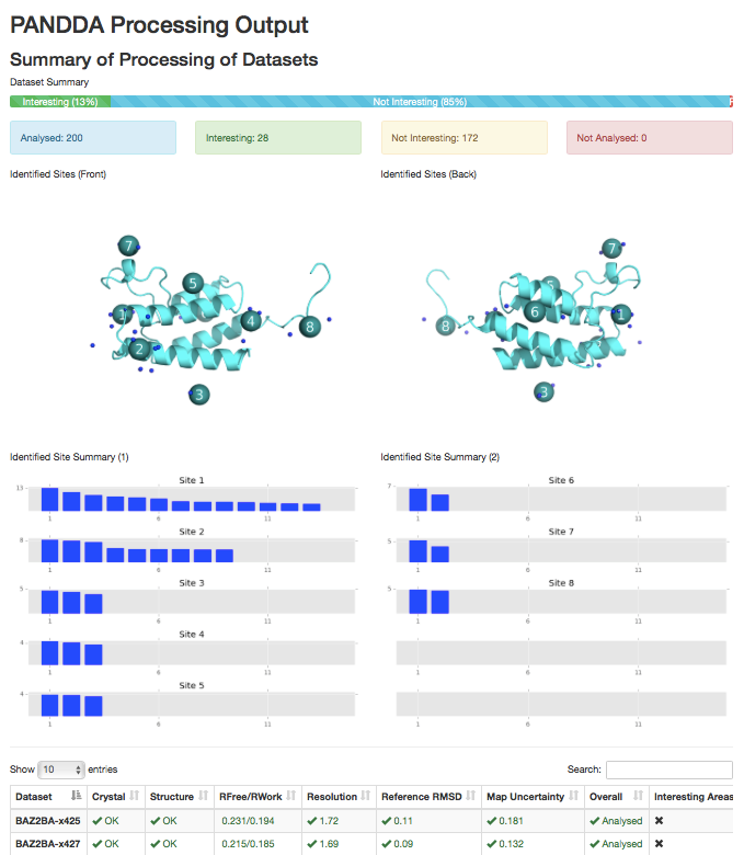
Images of the identified sites on the protein (requires pymol), and a site-by-site graph of the strengths of the identified events. Table of dataset parameters
3) pandda.inspect output summary.
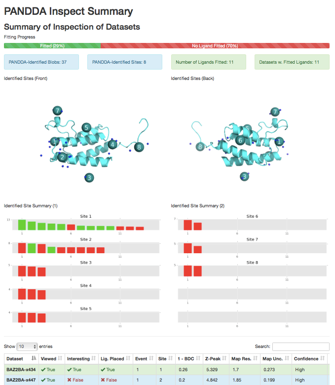
Images of the identified sites on the protein (requires pymol), and a site-by-site graph of the strengths of the identified events, coloured by whether a ligand marked was fitted. Table of dataset parameters, updated to include comments and meta-data about the fitting of the ligand.
After all of the modelling has been done, you must run the pandda.export script. For each dataset, this will take the newly-created model of the new conformation (the one present in the event map) and merge it with the original model from the ground state crystal.
pandda.export pandda_dir='./pandda' export_dir='./pandda-export'
will export all of the datasets from './pandda' and output them into a folder './pandda-export'. By default, this will export any dataset where a minor conformation has been modelled (when a model has been saved from the pandda.inspect GUI).
It is possible to filter the modelled structures, and only export particular datasets.
pandda.export pandda_dir='./pandda' export_dir='./pandda-export' select_datasets=JMJD2DA-x005,JMJD2DA-x007
will export only datasets JMJD2DA-x005 and JMJD2DA-x007 (again, these datasets must have a model saved to be exported). Multiple "select_datasets=" can be given. In this case, if no "option=" is given, then the argument is assumed to be a dataset label for export, so the "select_datasets=" may be omitted, making this
pandda.export pandda_dir='./pandda' export_dir='./pandda-export' JMJD2DA-x005 JMJD2DA-x007
By default, pandda.export exports the input PDB and MTZ file, the pandda (newly modelled) conformation, the ensemble model, any ligand files, the Z-maps and Event maps.
Partial-occupancy "weak" ligands always have a superposed ground-state conformation
When a ligand is present at less than near-full occupancy (certainly when the ligand is in less than ~80% of the unit cells of the crystal) it is necessary to have a superposed model that represents the solvent in the remaining unit cells. This superposition is required for the refinement program to achieve a good refinement, otherwise the ligand will try to fill the density for the solvent, leading to a poor and potentially incorrect ligand model.
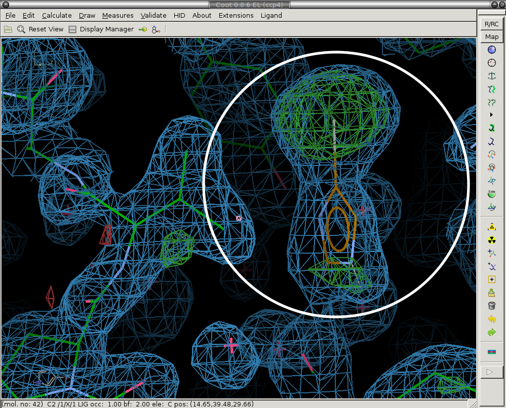
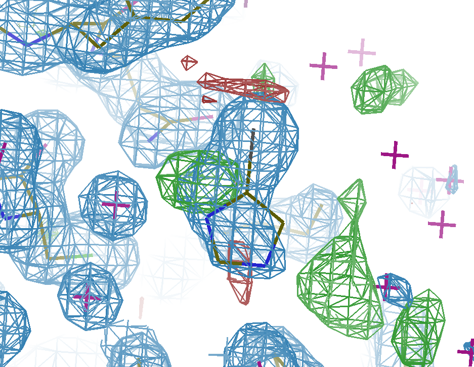
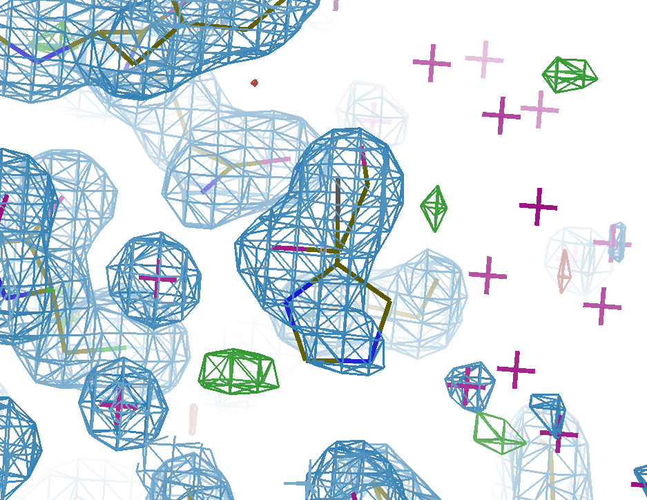
As an example, consider the structure below. The density for the ligand in the event map is clear (left), but there are blobs of density in the normal 2Fo-DFc map (centre) that are unexplained by the ligand model alone -- these are caused by the superposed solvent. Refining the ligand as an ensemble with the already-known unbound state (an ethylene glycol molecule) leads to a good model with all of the density explained (right). See our paper on the use of multiple states in ligand modelling for more details.
PanDDA Event Map
(showing the density for the ligand model)

Full Crystallographic Dataset
(refined with the ligand model only)
Full Crystallographic Dataset
(refined with the multi-state model)
You should therefore always use an ensemble model for refinement.
Partial-occupancy "weak" ligands may not be visible in the normal crystallographic maps
For-low occupancy ligands, there will be little or no visible trace of the ligand in the full dataset maps. This is because the superposed ground-state obscures the density for the ligand. It does not mean that the ligand model is incorrect.
Overview of the multi-state modelling and refinement protocol
pandda.export automatically generates an ensemble model by merging the original dataset structure with the newly modelled conformation from pandda.inspect. pandda.export will give the ligand-bound conformation an alternate conformer id (e.g., C,D), and will give the ground state conformer another id (e.g. A,B). This ensemble model is used for refinement. Inbetween refinement cycles, you should split the ensemble model back into the bound-/ground-state models and model each separately (see below).
The four stages that make up the multi-state refinement protocol are also brielfy described below, starting from just after pandda.export.
1) Generation of restraints for refinement (giant.make_restraints)
To stabilise refinement and make the models physical, giant.make_restraints can automatically identify groups of residues whose occupancies should be the same. giant.make_restraints makes occupancy contraints by identifying local groups of residues with same conformer. Residues will only be grouped together if they have the same conformer ID. The output restraint files can then be fed to giant.quick_refine, which then either runs phenix or refmac (see below).
giant.make_restraints ensemble.pdb
2) Quick-and-easy refinement (giant.quick_refine)
To make refinement more straightforward, giant.quick_refine can be used to refine the models. This organises the input and output files for each refinement into directories, and can also automatically generate and use the occupancy groupings described above. Use of giant.quick_refine is described in the options page, but a normal refinement will look like
giant.quick_refine input.pdb input.mtz ligand.cif restraints.params
... replacing the filenames with the appropriate names.
3) Splitting the ensemble model (giant.split_conformations)
Manipulation of the ensemble model can be tricky: where multiple conformations are present, it quickly becomes confusing which states belong to the bound-/ground-state conformations of the protein.
Therefore, after refinement, we split the models into two structures, one for the bound conformations (those in the event map), and those in the ground state (from the reference dataset/input model).
giant.split_conformations refined.pdb
4) (Re-)modelling of the bound-/ground-states (coot)
The amount of modelling that needs to be done after pandda.export often depends on the quality of the reference model (especially for weaker ligands). To minimise the amount of work required, it is highly recommended to use a strucuture that is as complete as possible as the input to pandda.
However, if modelling is required, the bound and ground states are modelled separately (e.g. in coot):
- The ground-state conformations should be modelled into a ground-state ("reference") dataset/map (e.g. "*-ground-state-average-map.native.ccp4" from pandda.analyse).
- The bound-state conformations of the protein are modelled into the appropriate event maps, as in pandda.inspect.
However, if you want to edit both structures simultaneously (e.g. to add a molecule that is the same in both states), then this should be done to the combined ensemble model.
5) Re-merging single-state models for refinement.
After you have re-modelled the bound- and ground-states of the protein, you need re-assemble the ensemble model for refinement.
giant.merge_conformations ground-state.pdb bound-state.pdb
You then generate restraints and refine as in steps 1) & 2); continue modelling and refining until you are happy/bored.
There are many criteria that can be used to validate ligand models. Many of these criteria are ignored due to beliefs in a subjective interpretation of the density. However, given the clarity of the event maps, these criteria can now be used to highlight potential errors in the models which can lead to meaningful corrections. In this way, outliers can more confidently be regarded as features of the model, rather than errors in the model.
RSCC |
Real-Space Correlation Coefficient | Correlation between the model and observed density. A correlation of >0.7 is generally required for a "good" model. This measure has resolution dependence, and can also be expected to decrease for low occupancy models. However, for high resolution models, a value of <0.7 probably indicates problems with model. |
|---|---|---|
RSZD |
Real-Space Difference Z-Score | Statistical significance of the difference density for the measured residue. Values >3 indicate significant amounts of difference density and should be investigated. |
RSZO |
Real-Space Observed Z-Score | Strength of the density for the measured residue. This is a signal-to-noise ratio, so low values <1 may indicate that there is no density to support the ligand's presence. |
B-Ratio |
Ratio of ligand/protein B-factors | Ratio of the ligand's B-factors to the surroundings. Ligands are normally more mobile than the protein side-chains in contact with the ligand, so this values will normally be >1. However, for values >>2, it is unlikely that the ligand has been modelled/refined correctly, and so such ligands should be investigated and re-refined, re-modelled or deleted. |
RMSD |
Movement of ligand after refinement | Measure of the difference between the coordinates of the initial and the refined model of the ligand. Large values of RMSD, indicate that the model has moved significantly since it was placed. If density is good for the ligand, you would expect only small movements (<1). |
Large values of B-factors and small values of RSZO are not necessarily indicative of errors in the model, but may simply highlight very weak features. If strong evidence is seen in the event map for binding, then it may be possible to conclude that these are real features of the data, rather than errors in the model.
Small values of RSCC, and large values of RSZD and RMSD, however, should not be ignored, as these indicate significant disagreement between the data and the model. Large values of RMSD should only be accepted when the user has intentionally changed the model, such as flipping a group through 180° to gain better bonding networks.
There is a script available called giant.score_model that can be used to score ligands. It is designed to be used with the output of pandda, but can in theory be used on any model. This script scores the final refined model against the final refined density, and against the initial refined density (before the placement of the ligand). It also compares the final refined structure to the inital model (with the initial placement of the ligand). The script generates all of the scores above using the EDSTATS script, and outputs radar plots for each analysed residue.
The normal usage of giant.score_model on files from panddas is
giant.score_model pdb1=refine.pdb mtz1=refine.mtz pdb2=<label>-ensemble-model.pdb mtz2=<label>-pandda-input.mtz
where refine.pdb and refine.mtz are the output from the most recent round of refinement, and the other files are from pandda.export. <label> is the label of the dataset.
It is also possible to run giant.score_model_multiple to score all models in the pandda.export folders. The defaults for this script are the same as the files used above, and is the recommended way to use this script.
giant.score_model_multiple out_dir="./validation_images" /path/to/pandda/export/directory/*
will output images for every folder in /path/to/pandda/export/directory. Folders can also be specified individually if required. The name of each folder is used to label the dataset.
Several examples of the output are shown below:
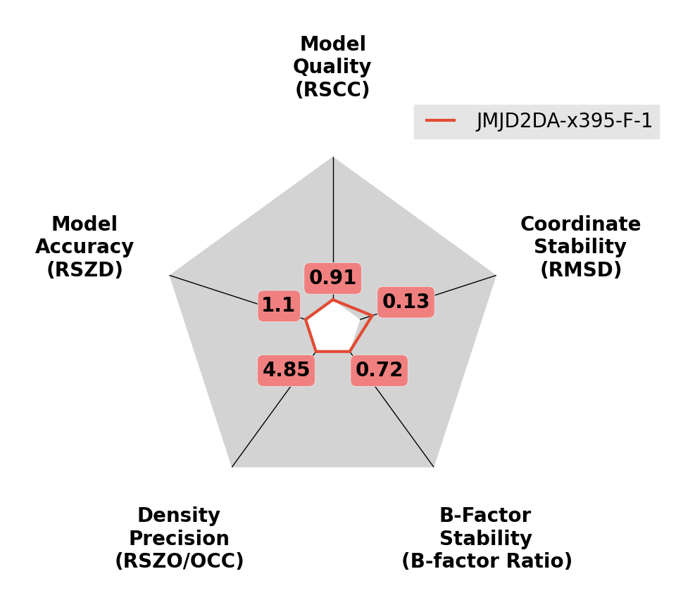
A high-quality ligand model.
Scores are all good, so that the lines remain close to the centre of the plot.
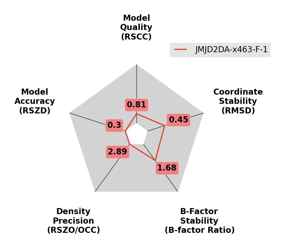
A reasonable quality ligand model.
B-factors are slightly inflated and ligand moves from inital pose during refinement.
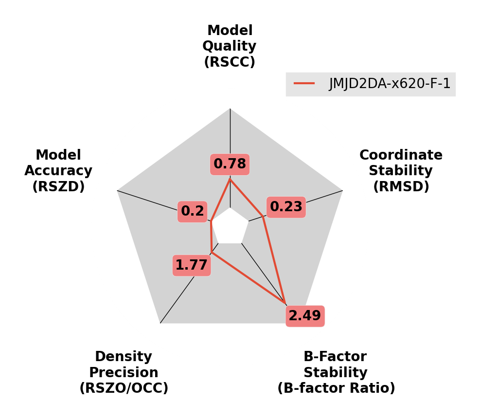
A ligand with high B-factors.
The B-factors of this ligand are much higher than the surroundings. Try reducing the occupancy of the ligand and resetting the B-factors, before refining again.
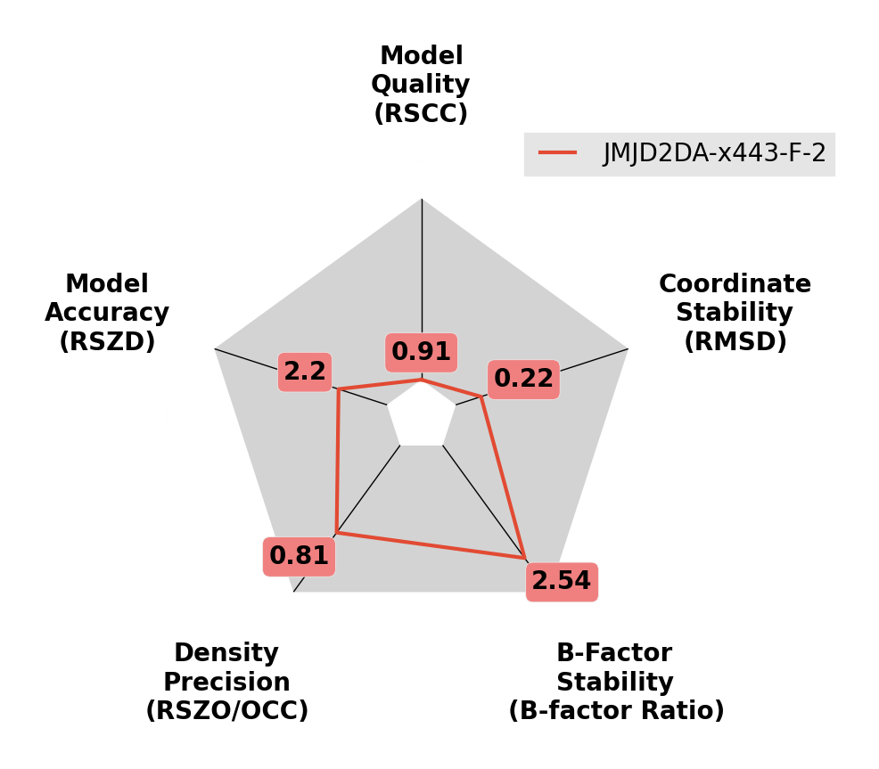
Imbalance in occupancy and B-factors.
The density for the ligand is weak (as given by RSZO), and the B-factors are large. Try reducing the occupancy of the ligand and resetting the B-factors, before refining again.
Which models do I deposit?
For deposition in the PDB, you MUST deposit the ensemble model from the last round of refinement.
For chemists and for structural analysis, it's normally easier to inspect the models after splitting.